A transistor works as an amplifier that can control the conversion of energy and amplify the output without distortion of any small changes in the input. For example, in the amplification process of the transistor, the input signal is a small current, and through the diffusion process of the base region, the output current can become very large to drive other electronic devices. Next we will analyze this type of circuit in detail.
Transistor Amplifier Circuits
Basic
For transistor amplifier circuits, they are generally a mixture of DC and AC. During analysis, it is necessary to analyze them separately, so DC analysis and AC analysis are included.
1) For DC path, include follow the following rules:
a. The capacitor is considered an open circuit, that is, the capacitor is disconnected.
b. The inductor is treated as a short circuit, i.e. replaced by a wire.
c. The voltage source is short-circuited, the current source is open-circuited, and the internal resistance remains.
2) For AC path, include follow the following rules:
a. Large capacitance is considered a short circuit.
b. A DC power supply without internal resistance is considered a short circuit.
c. The DC voltage change is 0, which is regarded as a short circuit.
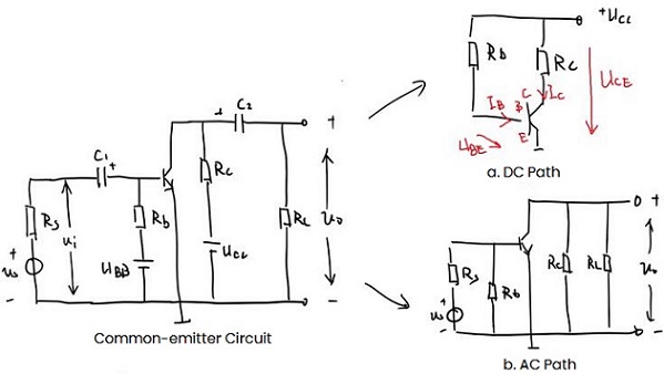
Figure 1: Basic Transistor Amplifier Circuit
Static Analysis
1. Graphical Method
Redraw the above DC path to get the relationship between iC and uCE.
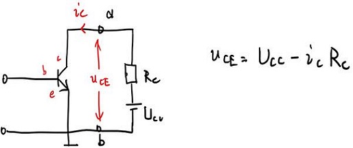
Figure 2: DC Path 1
According to the above formula, determine the two points to get the DC load line, and put the DC load line into the output characteristic curve.
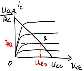
Figure 3: Output Characteristic Curve
Usually we find IBQ through the DC path base circuit to know the determined characteristic curve
IBQ=(UCC-UBE)/Rb. The UBE of the Si tube is 0.6V- 0.7V, and the Ge tube is 0.2V- 0.3V.
2. Analytical Method
The first step is to draw the DC path, as follows:
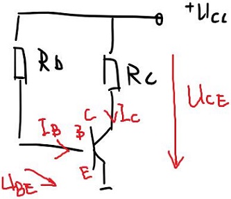
Figure 4: DC Path 2
The calculation order is: IB→IC→UCE
1) IB is equivalent to IBQ, and IBQ=(UCC-UBE)/Rb=UCC/Rb
2) IC=βIB
3) UCE=UCC-IC*RC
Effect of Circuit Parameters on Static Operating Point
Using the common emitter circuit diagram as a reference, explore the effects of Rb, Rc, and UCC on the static operating point. When one parameter changes, the other two remain unchanged:
1) Rb increases and moves downward along the load line, otherwise it moves along the load line.
Since Rb changes affect IBQ but not the load line, the load line actually remains unchanged while the IBQ in the output characteristic curve moves up or down. That is, as Rb increases and IBQ decreases, the operating point moves downward, and vice versa.
2) As Rc decreases, the operating point moves to the right, otherwise move to the left.
From the formula of the DC load line we can see that Rc is actually its slope. As Rc decreases, the load line becomes steeper, so the operating point moves to the right, and vice versa.
3) Ucc increases, the DC load line moves upward in parallel, and the operating point moves to the upper right, otherwise, move to the lower left.
Changes in Ucc affect both the DC load line and the IBQ in the characteristic curve. When UCC increases, IBQ increases, and the curve moves upward; and there is UCC in the intercept of the DC load line, so the DC load line moves upward in parallel. Finally, the operating point moves to the upper right.
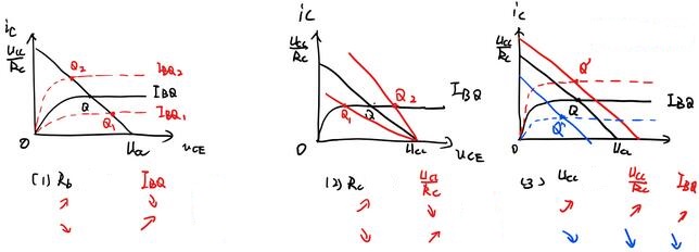
Figure 5: Characteristic Curve Changes
Dynamic Analysis
1. Graphical Method
Similar to static analysis, the operating state of the transistor moves along the AC load line. Here the first step is to make the AC load line.
Two characteristics of AC load lines:
1) It must pass through the static working point. When the AC signal is 0, the input signal at this time is only a DC signal, which is a static operating point.
2) The slope is represented by -1/RL’, where RL’=Rc//RL (Rc and RL are connected in parallel)
Therefore, the AC load line can be made by the following steps:
1) Make an auxiliary line based on the slope.
2) Find the static operating point Q.
3) Draw a straight line through Q parallel to the auxiliary line, which is the AC load line.
4) Use AC load lines to draw current and voltage waveforms, or find the maximum undistorted output voltage.
After determining the Q, the AC load line can also be determined by the intercept of the AC load line on the uCE axis: intercept Ucc’=UCEQ-ICQ*RL’
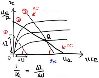
Figure 6: Intercept
Next, we determine the AC waveform. Since electrical signals contain DC signals and AC signals, we get the following formula:
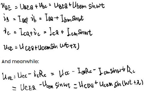
The base current ib, the collector current ic and the collector voltage ube have the same phase, while uce is different, that is, the output voltage has the opposite phase to the input voltage. It can be seen from the above formula that the signal entering from the outside is basically unchanged after reaching b, and the signal entering from c is basically unchanged. But the signal flowing out from e becomes reverse, and finally this reverse signal is amplified and output.
2. Nonlinear Distortion
Mainly divided into the following three types:
1) Saturation distortion: The operating point reaches the saturation zone.
2) Cutoff distortion: The operating point reaches the cutoff area.
3) Bidirectional distortion: When is the operating point, but the signal is too large, causing the peaks and troughs to be cut off.
* Distortion due to non-linearity of the characteristic curve
The input characteristic curve is actually bent and then shows a linear growth trend. However, if the input uBE is too small, part of the IB will be in the curved interval and the other part will be in the linear interval, resulting in distortion. Usually the intervals of the output characteristic curves are the same, but when they are different, such as sparse at the top and dense at the bottom, distortion will also occur.
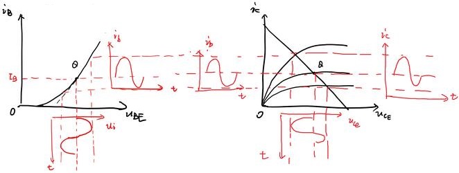
Figure 7: Distortion Due to Non-linearity of The Characteristic Curve
* Distortion caused by inappropriate static operating point
Mainly include saturation distortion and cutoff distortion. The saturation distortion is due to the static operating point being set too high, when ib increases, ic will not increase accordingly, and the output voltage uCE will have bottom distortion. During cut-off distortion, because the static operating point is set too low, the negative half cycle of the input signal enters the cut-off area, and the output voltage uCE appears top-distorted.
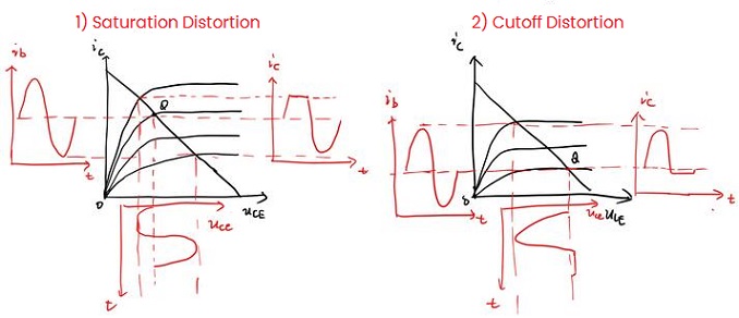
Figure 8: Saturation Distortion and Cutoff Distortion
In order to avoid the occurrence of the above distortion, we introduce the maximum undistorted output voltage Umax, that is, the peak-to-peak voltage Up-p: When the static operating point is determined, the input signal is gradually increased, and the transistor neither enters the saturation zone nor the cut-off zone, then the maximum output voltage obtained.
3. Microvariant Equivalent Circuit
When the signal change range is very small, it is considered that the changes in the transistor voltage and current are linearly related, that is, the input characteristics and output characteristics can be regarded as straight lines. So a linear model is used to replace the transistor and placed in the circuit to form a slightly variable equivalent circuit. Here, iB and uCE are used to represent uBE and iC, and then differentiation is performed. Note that each quantity here is the sum of the AC component and the DC component, but the change of the DC component is 0, so it is still 0 after differentiation. Then use h11, h12, h21, h22 to replace the differential components, and there is the following formula:
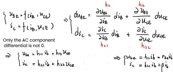
Analyze each h in terms of units
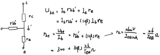
1) h11 is the output AC short-circuit resistance, expressed in rbe, and is estimated as follows:
2) h12 is a constant, which is called the voltage feedback coefficient μr when the input AC is open circuit.
3) h21 is a constant, called the current amplification coefficient β when the output AC short circuit occurs, and is usually given directly (product manual).
4) h22 is the admittance when the input AC is open circuit, expressed as 1/rce.
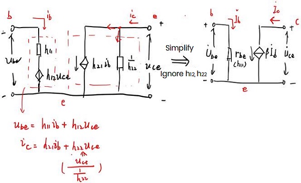
Figure 9: Circuit Simplification
Have to be aware of some tips:
1) Equivalence is only for microvariables (AC small signals). The external DC power supply should be set to zero (voltage source short circuit, current source open circuit), and the parts related to micro variables should be retained.
2) The value and direction of the controlled current source βib in the equivalent circuit depend on the base current ib, and the current direction of ib cannot be changed at will. If ib flows into the base, then βib flows from the collector to the emitter (as shown in the figure). Otherwise, it flows from the emitter to the collector.
3) The microvariable equivalent circuit is only suitable for low-frequency, small-signal transistors.

 English