How Do Sequential Data and Linked Data Structure Formed?

The data can be access either sequentially or randomly in computer. If access, how to find them exactly? How is the data stored in the computer? in what form? In a computer, data information is not isolated and disordered, but as a data set with intrinsic connections. Among them, one or more specific relationships exist between data elements. In order to write a good program, it is necessary to analyze the characteristics of the objects to be processed and the relationship between them. This is what it means to study data structures. Here we will talk sequential storage structure and linked storage structure.

Data Structure

Data structure is a way for computers to store and organize data. It is a collection of data elements that have one or more specific relationships with each other. According to different views, we can roughly divide data structures into two types: physical structure and logical structure.

Logical Structure

This data structure reflects the logical relationship between data elements, not their storage location in the computer.

Set: The elements in the data structure have no other relationship except "belonging to the same set".

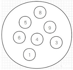
Figure 1: Data Set

Linear structure: There is a one-to-one relationship between elements in the data structure.

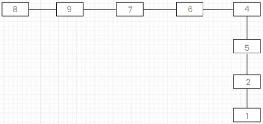
Figure 2: Linear Structure

Tree structure: The elements in the data structure have a one-to-many relationship.

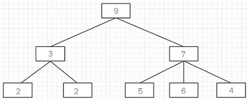
Figure 3: Tree Structure

Circular structure: Elements in it have a many-to-many relationship.

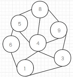
Figure 4: Circular Structure

Physical Structure

It is also called the storage structure, which refers to the storage form of the data in the computer. In other words, it actually means how to store the data elements in the memory of the computer. Storage is mainly for internal memory, and the data organization of external storage such as hard disks, floppy disks, and CDs is usually described by a file structure.

The storage structure of data should correctly reflect the logical relationship between data elements, which is the most critical. How to store the logical relationship between data elements is the point.

There are two storage structures for data elements: sequential storage and chained storage.

Sequential data structure: Data elements are stored in memory cell units with continuous addresses, and the logical and physical relationships between the data are consistent.

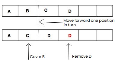
Figure 5: Sequential Data Structure

Linked data structure: It is to store data elements in any storage unit, and the storage units can be continuous or discontinuous in a set. The storage relationship of data elements does not reflect its logical relationship, so a pointer needs to be used to store the address of the data element, so that the location of the associated data element can be found through the address, which is much more flexible.

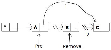
Figure 6: Linked Data Structure

Arrays

An array is a sequential structure in terms of physical structure, but a linear structure in terms of logical structure. An array is a data set of the same type that is stored continuously in memory. There are heaps and stacks in the JVM, where a continuous storage means that the data in the array is arranged consecutively in the heap. This is what the array is in s representation in memory.

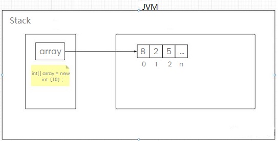
Figure 7: JVM

Array Query

The query of the array is calculated by a formula: a[n] = start address + (n * number of bytes), and n represents the subscript. For example, if we want to find a subscript 2 at this time, then use the formula to calculate, 100 + (2*4), then you will find the element whose address is 108, that is, 5, because it has a formula, after calculation, you can quickly find the address of this element, and the query time is complicated, which is O(1). In this case, finding the subscript is also called random access.

1) The array supports random access, and the time complexity of random access according to the subscript is O(1).

2) When the array is sorted, the time complexity of the array is O(logn) when binary search is used.

3) In the case of sequential search of the array, each element needs to be traversed until they are equal, and then returned, so the time complexity is O(N).

Array Insertion

1) If the tail insertion method is used, the time complexity is O(1), because it does not involve the movement of other elements.

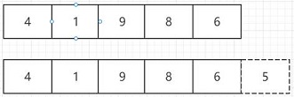
Figure 8

2) If the head insertion method is used, the time complexity is O(N), because each element of the array has to be moved backwards.

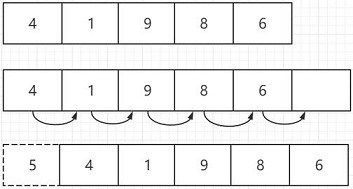
Figure 9

3) If you insert in the middle, the time complexity is also O(N), because the elements behind the insertion position also need to move backward.

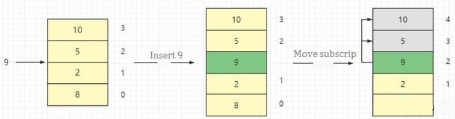
Figure 10

Array Deletion

1) If the head deletion method is used, the time complexity is O(N), because other elements need to be moved forward one bit.

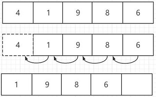
Figure 11

2) If the tail deletion method is used, the time complexity is O(1), which does not involve the movement of other elements.

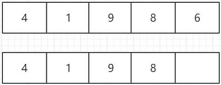
Figure 12

3) If it is middle deletion, the time complexity is also O(N), because the element after the deleted position has to be moved forward one bit.

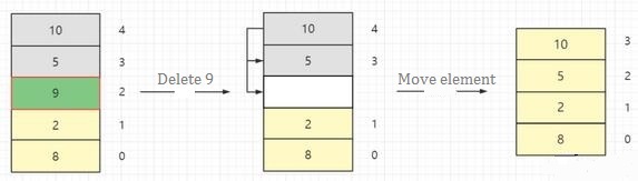
Figure 13

Dynamic Arrays

The data we analyzed above are normal and one-dimensional arrays. Next, we analyze dynamic arrays, also known as augmentable arrays, variable-length arrays, dynamic tables, and array tables. They are random-access and automatic linear data structure with the ability to add or remove elements.

An easy way to implement a dynamic array is to first initialize the array with a fixed size. Once the array is full, create a new array 1.5 times the size of the original array (copying the old array data into the new one). Likewise, if the number of elements stored in the array is less than half the size of the array, the size of the array is reduced by half.

1) The time complexity of dynamic array header insertion is O(N), because it will involve other elements moving backward or expanding.

2) If the time complexity of dynamic array tail insertion is not expanded, then it is O(1), and if it needs to be expanded, then it is O(N).

3) Insertion in the middle of the dynamic array, the time complexity is O(N), because it will involve the movement of other elements or the expansion of the array.

1) Time complexity of dynamic array head deletion is O(N), because it will involve other elements moving forward or shrinking.

2) The time complexity of dynamic array tail deletion, if shrinkage is considered, then the time complexity is O(N), otherwise it is O(1).

3) The time complexity of deletion in the middle of the dynamic array is O(N), because it will involve moving forward or shrinking other elements.

The situation for dynamic array queries is the same as for normal arrays.

When adding elements, the capacity of the old array is not enough. At this time, the old array cannot be expanded directly, because the capacity of the old array is determined. Then it is necessary to create a new array and move the elements of the old array into the new array.

Proceed as follows:

1) Determine whether the capacity is sufficient, that is, size + 1 <= elements.length, where elements represent the old array.

2) Create a new array newElements with a capacity 1.5 times that of elements (it is more efficient to use bit operations).

3) Move the elements to newElements.

4) Point the newElements.

When deleting elements, there will be fewer and fewer elements in the old array. When the number reaches a certain level, the original space of the array will be wasted, so the shrinking operation is necessary. At very first, you need to create a new array, and move elements from the old array to the new array.

Proceed as follows:

1) Judging whether the capacity is sufficient, that is, when the size is greater than half of the capacity of elements, or when the capacity is less than the default capacity of DEFAULIT_CAPACITY 10, there is no need to perform shrinking operations.

2) Create a new array newElements with a capacity of 1/2 of elements (it is more efficient to use bit operations).

3) Move the elements to newElements.

4) Point the newElements.

Linked List

Introduction

It belongs to the chain structure in terms of physical structure, and also belongs to the linear structure in terms of logical structure. Linked list includes singly linked list, doubly linked list, circular linked list and so on. Compared with the linear list, adding and deleting operations are very convenient, because there is no need to move a large number of nodes, only need to modify the corresponding front and rear node pointers. As a linked list, the node must also add the next node pointer in addition to the basic info. It is convenient for the computer to search in the memory. We usually call the field storing basic info a data field, and the field storing the direct successor position a pointer field. The storage image of data elements composed of these two parts is called a node. The first point is called the head node or the dummy node, the second node belongs to the real first node, which can store nothing, or store some public data such as the length of the linked list information.

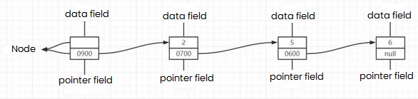
Figure 14: Linked List

It contains multiple nodes, and each node has a next pointer pointing to the successor element, and the value of the next pointer of the last node is null, indicating the end of the linked list.

Figure 15

Each data node in it has two pointers, which point to the direct successor and direct predecessor respectively. Therefore, starting from any node in the doubly linked list, you can easily access its predecessor node and successor node.

Figure 16

Changing the pointer end of the terminal node in the singly linked list from a null pointer to pointing to the head node makes the whole singly linked list form a ring.

Figure 17

Insertion and Deletion

For Singly Linked List

Head Insertion

If you need to insert a new node in the current header node, you only need to modify a next pointer, which can be done in two steps:

* Modify the next pointer of the new node to point to the current header node.

Figure 18

* Change the value of the header pointer so that it points to the new node (the previous header pointer pointed to 15, and it points to the new data after modification).

Figure 19

Tail Insertion

If you need to insert a new node at the end node, you need to modify two pointers (the next pointer of the last node and the next pointer of the new node), which can be done in two steps:

* The next pointer of the new node points to NULL.

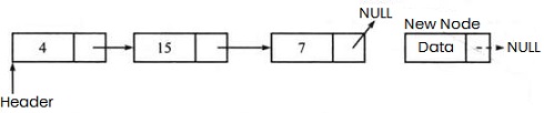
Figure 20

* The pointer of the last node points to the new node.

Figure 21

Middle Insertion

Assuming that the position of inserting a new node is given, in this case, two pointers need to be modified. If an element is to be added at position 3, the pointer needs to be positioned at position 2 of the linked list, that is, two pointers need to be passed from the head of the list node, and then insert a new node, for simplicity, assume that the second node is a position node.

* The next pointer of the new node points to the next node of the position node.

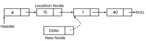
Figure 22

* The next pointer of the position node points to the new node.

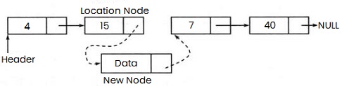
Figure 23

If the head insertion method is used, the time complexity is O(1), otherwise it is O(N), and no matter which way the insertion space complexity is O(1).

Head Deletion

Deleting the first node from the linked list can be achieved in two steps:

*Create a temporary node, which points to the node pointed by the header pointer.

Figure 24

*Modify the value of the header pointer so that it points to the next node, and remove the temporary node (before deletion, the header pointer points to 15, after it, the header pointer points to 7).

Figure 25

Tail Deletion

The last node is deleted, which is a little more complicated than deleting the head node of the linked list. Because it needs to find the predecessor node of the tail node, and it is implemented in three steps.

* When traversing the linked list, it is necessary to save the address of the predecessor (the previous pass) node when traversing. And for the end of the linked list, there will be two pointers, namely the pointer to the end node and the pointer to the end node pointer to predecessor node.

Figure 26

* Update the next pointer of the predecessor node of the tail node to NULL.

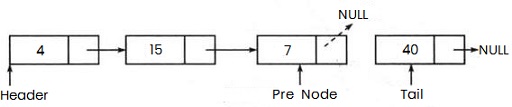
Figure 27

Remove the tail node.

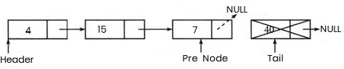
Figure 28

Middle Deletion

In this case, the node to delete is always between two nodes, so there is no need to update the pointers of the head and tail. This operation can be realized in two steps.

* Save the address of the predecessor (the previous pass) node during traversal. Once the node to be deleted is found, update the value of the next pointer of the predecessor node to the value of the next pointer of the deleted node.

Figure 29

* Remove the current node that needs to be deleted.

Figure 30

Under this way, the time complexity is O(1), otherwise it is O(N), and no matter which way the insertion space complexity is O(1).

For Doubly Linked List

Head Insertion

In this case, it is necessary to modify the values of the predecessor pointer and the rear pointer.

*Update the successor pointer of the new node to point to the current header node, and assign NULL to the predecessor pointer of the new node.

Figure 31

* Update the predecessor pointer of the header node to point to the new node, and then use the new node as the header.

Figure 32

Tail Insertion

In this case, it is necessary to traverse to the end of the linked list, and then insert a new node.

* The successor pointer of the new node points to NULL, and its predecessor pointer points to the end node.

Figure 33

* Update the right pointer of the last node to point to the new node.

Figure 34

Middle Insertion

Need to traverse the linked list, know the position node, and then insert the new element.

* The successor pointer of the new node points to the successor node of the node where the new node needs to be inserted. Then make the predecessor pointer of the new node point to the location node.

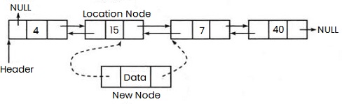
Figure 35

*The predecessor pointer of the successor node of the position node points to the new node, and the successor node of the position node points to the new node.

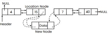
Figure 36

Head Deletion

In this case, delete the first node (the current head node) from the doubly linked list. This operation can be achieved in two steps:

* Create a temporary node, which points to the same node as the header.

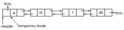
Figure 37

* Modify the header node pointer head to make it point to the next node, change the predecessor pointer of the header node to NULL, and then remove the temporary node.

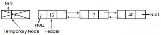
Figure 38

Tail Deletion

The handling of this way is more complicated than deleting the first node of the doubly linked list, because the predecessor node of the tail node must be found. It takes 3 steps to achieve:

* Traverse the linked list, and save the address of the predecessor (the previous pass) node when traversing. And for the end of the table, there are two pointers, which are the tail pointer pointing to the tail node and the pointer pointing to the predecessor node of the tail node.

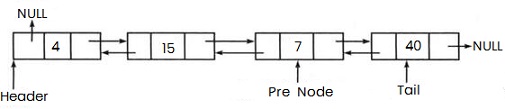
Figure 39

* Update the next pointer of the predecessor node at the end of the list to NULL.

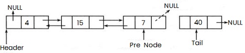
Figure 40

* Remove the end node.

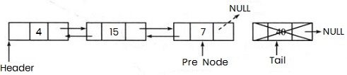
Figure 41

Middle Deletion

In this case, the node to delete is always located between two nodes, so the values of the head and the tail do not need to be updated. And this can be achieved in two steps:

* Similar to the previous method, the pre node is saved when traversing the linked list. Once the node to delete is found, change the next pointer of the pre node to point to the next node of the deleted node, and change the previous pointer of the successor node of the deleted node to point to the pre node.

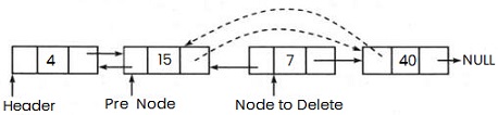
Figure 42

* Remove the current node being deleted.

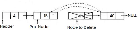
Figure 43

For Circular Linked List

Head Insertion

The only difference between head insertion and tail insertion is that the pointer needs to be updated after inserting a new node. The specific steps are as follows:

Figure 44

* Create a node, and initialize its next pointer to point to the node's own head node, and then traverse the linked list to the end. That is, the insertion position should be the node position where the next node in the list is the header node (this node is the pre node of the header).

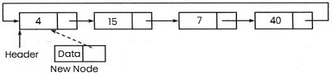
Figure 45

* Update the next pointer of the pre node of the header to point to the new node, and obtain the following list as shown in the figure below.

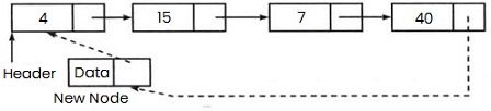
Figure 46

* Set the new node as the header node.

Figure 47

Tail Insertion

Insert a node containing data at the tail starting from the head. The new node will be placed behind the tail node, that is, the new node will be inserted between the tail node and the first node.

* Create a node, and initialize its next pointer to point to the node itself.

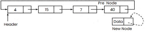
Figure 48

* Update the next pointer of the new node as the head node, and then traverse the circular linked list until the end of the list. That is, the insertion position should be the node position where the next node is the header node (this node is the pre node of the header).

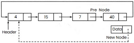
Figure 49

* Update the next pointer of the pre node of the header to point to the new node, and get the circular linked list as shown in the figure below.

The time complexity is O(N), which is used to scan a linked list of length N, and the space complexity is O(1).

Figure 50

Head Deletion

The operation of deleting the first node is very simple, just point the next pointer of the tail node to the successor (next) node of the first node.

* Traverse the linked list to find the tail node, which is the pre node of the header node to be deleted.

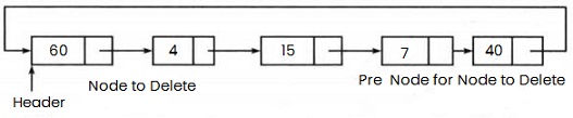
Figure 51

* Create a temporary node pointing to the header node. Update the next pointer of the tail node so that it points to the successor node of the first node.

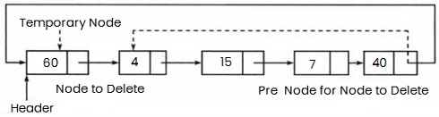
Figure 52

* Modify the value of the head pointer to make it point to the successor node, and remove temporary nodes.

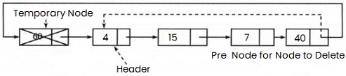
Figure 53

Tail Deletion

In order to delete the last node in the circular linked list, it is necessary to traverse the linked list to the penultimate node. This node will become the new tail node, and its next pointer will point to the first node of the linked list. Take the linked list in the figure below as an example. In order to delete the last node 40, first traverse the linked list to node 7, then point the next pointer of node 7 to node 60, and rename this node as the end of the list.

* Traverse the linked list to find the tail node and its pre node.

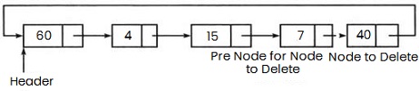
Figure 54

* Update the next pointer of the pre node of the tail node so that it points to the head node.

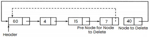
Figure 55

* Remove the tail node.

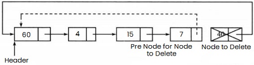
Figure 56

Under this way, the time complexity is O(N), which is used to scan a linked list of length N, and the space complexity is O(1).

Sequential Data Structure vs Linked Data Structure

1. Based on storage space

The storage space of the sequence table is allocated statically, and its storage size must be clearly specified before the program is executed. The linked list does not need to estimate the storage size in advance, but the storage density of the linked list is low.

The storage density of the sequential storage structure is 1, while the storage density of the chain storage structure is less than 1.

2. Based on calculation

The time complexity of accessing by serial number in the sequential list is O(1), while the time complexity of accessing by serial number in the linked list is O(N).

3. Based on the environment

Sequence tables are easy to implement. There are array types in any high-level language. The operation of linked lists is based on pointers, relatively speaking, sequence tables are simpler.

In short, the two storage structures have their own advantages, and which one to choose depends on the actual problem. Generally speaking, sequential storage is selected for more stable linear tables, and linked storage is more suitable for linear tables with frequent insertion and deletion operations.