RLC Circuit - Basics, Calculation, Oscillation Explained

The RLC circuit is a common electronic circuit that used to control and regulate current and voltage. It is widely used in various fields, including communications, power supplies, filters, oscillators, etc. Different connection methods and parameter selections give RLC circuits a variety of functions and characteristics. Understanding the concept, classification, and functions of RLC circuits is very important for understanding and designing electronic systems.

What is RLC Circuit?

1. Basic Concepts

RLC circuit refers to a circuit composed of three basic components: a resistor (R), an inductor (L) and a capacitor (C). These components have different electrical properties and behaviors respectively, and their combination forms the specific functions and characteristics of the RLC circuit.

R: A resistor is a component that consumes electrical energy and converts it into heat energy. Its main function is to limit the flow of current and control the voltage and power in the circuit by producing a resistance drop.

L: An inductor is a component that stores electrical energy. It creates a magnetic field by winding a wire or coil, and when the current changes, it produces a reverse electromotive force. And it plays a role in suppressing rapidly changing currents and filtering in circuits.

C: A capacitor is a component that stores electrical energy. It is separated by an insulating medium between two charged plates and can store electrical charges. Capacitors have the ability to store and release electrical energy in circuits and also play an important role in frequency selectivity and filtering.

By combining different R, L, and C components, various types of RLC circuits can be constructed to achieve different circuit functions and response characteristics.

2. Classification

According to the connection method and number of R, L, and C components used in the circuit, RLC circuits can be divided into the following common types:

Under this connection method, the current passes through the resistor, inductor and capacitor in sequence, and changes accordingly in each component. The series RLC circuit has the characteristics of frequency selectivity and presents different impedance and response characteristics at different frequencies, so it is widely used in filter circuits and tuned circuits.

2) In Parallel

Under this connection method, the current is divided in the branches and the voltage across each element is the same. The parallel RLC circuits have impedance characteristics for current at specific frequencies and can be used to selectively pass or block signals at certain frequencies.

A parallel-series RLC circuit provides more complex response characteristics, resulting in more flexible impedance and phase characteristics at different frequencies.

3. Function

1) Filter

According to the circuit characteristics and parameter selection, the RLC circuit can realize the functions of low-pass filtering, high-pass filtering, band-pass filtering or band-stop filtering. Filters are commonly used in communication systems to remove noise, adjust signal frequency range, and separate signals in different frequency bands.

2) Resonator

RLC circuits can be used as resonators, which can produce resonance phenomena at specific frequencies, because they can be made to have a larger impedance or current response at a specific frequency. This resonance phenomenon is widely used in radio communications, antenna design, oscillators and other fields.

3) Energy storage and transfer

Since both inductors and capacitors can store and release electrical energy, RLC circuits can be used for energy storage and transfer. The ability of inductors to store electrical energy has led to their use in DC-DC converters and power management, and capacitors are often used to smooth the output pulsations of power supplies, store energy, and provide additional power requirements.

4) Regulate voltage and current

By choosing appropriate component values and connections, the voltage and current values in a RLC circuit can be controlled to meet specific needs. This plays an important role in power management, voltage regulators, transformers, etc.

5) Delay and phase shift

Because inductors and capacitors introduce delay and phase shift effects, RLC circuits can be used to adjust the time response of signals. This is commonly used in communication systems for clock synchronization, signal processing in data transmission, etc.

Impedance of RLC Circuit (series)

1. Introduction

If a circuit consists of R1, R2, and R3, is its resistance easy to calculate? As shown in the figure below, R = R1 +R2+R3.

If a circuit consists of R, L, and C, what is its impedance? Is it also the accumulation of resistance and impedance?

It is stated in the book that when there are inductors and capacitors in a circuit, the circuit no longer exhibits pure resistor characteristics, but must be described by impedance.

Compared with resistance, impedance takes into account two factors:

1) The influence of the frequency of the input signal on the impedance.

2) Calculate the phase difference between voltage U and current I.

The impedance of a pure inductor is called "inductive reactance", represented by the symbol XL; the impedance of a pure capacitor is called "capacitive reactance", represented by the symbol XC. They are collectively called "reactance".

Ideally, resistors consume energy, while capacitors and inductors do not consume energy, but only convert energy. Because of this essential difference, resistance and reactance (capacitance/inductance) are mathematically represented by two-dimensional coordinates of an orthogonal coordinate system. The abscissa represents resistance, and the ordinate represents reactance. In particular, the positive half-axis represents inductance, and the negative half-axis represents capacitive reactance:

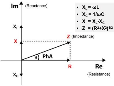
Figure 3: Impedance Coordinate System

Where, Z (impedance) can be expressed as a complex number, including two pieces of information: the module |Z| and the angle θ. However, in engineering, impedance often refers to |Z|. The calculation formula is listed in Figure 3.

The angle θ implies the phase information between voltage U and current I:

1) If it is a positive number, it means that the voltage U leads the current I in phase.

2) If it is a negative number, it means that the current I leads the voltage U in phase.

Let's sort it out. The current of the inductor cannot change suddenly, and the voltage changes first. The same is true for inductive circuits showing related characteristics (XL>XC). The voltage of the capacitor cannot change suddenly, and the current changes first. The same is true for  capacitive circuits showing related characteristics (XC>XL).

2. Impedance Calculation Case

In Figure 4, the R-L-C are 10Ω, 100μH, and 100μF respectively, where the input signal is 50Hz, and the peak amplitude is 10V. Calculate the circuit impedance and current effective values.

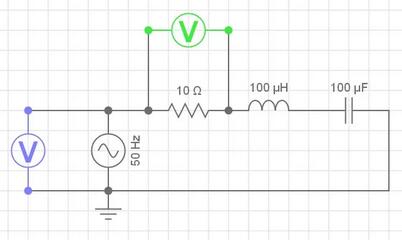
Figure 4: Impedance Calculation Case

XL=2π*fL=2*3.14*50*100^10-6=0.03Ω

XC=1/(2π*fC)=1/(2*3.14*50*100^10-6)=31.85Ω

X=XL-XC=-31.82Ω|Z|=(10^2+31.82^2)^(1/2)=33.35Ω

Irms=V(s-peak)*0.707/|Z|=10*0.707/33.35=0.212A=212mA

It should be noted here that calculating current or voltage through impedance is based on RMS (effective value), so a power supply with a peak amplitude of 10V needs to be multiplied by 0.707 to calculate the effective value. Because it is a series circuit, Irms is the same on all components. Let’s calculate the peak voltage amplitude on the inductor, capacitor, and resistor respectively:

V(L-peak)=V(L-rms)/0.707=Irms*XL/0.707=0.212*0.03/0.707=0.01V

V(C-peak)=V(C-rms)/0.707=Irms*XC/0.707=0.212*31.85/0.707=9.55V

V(R-peak)=V(R-rms)/0.707=Irms*R/0.707=0.212*10/0.707=3V

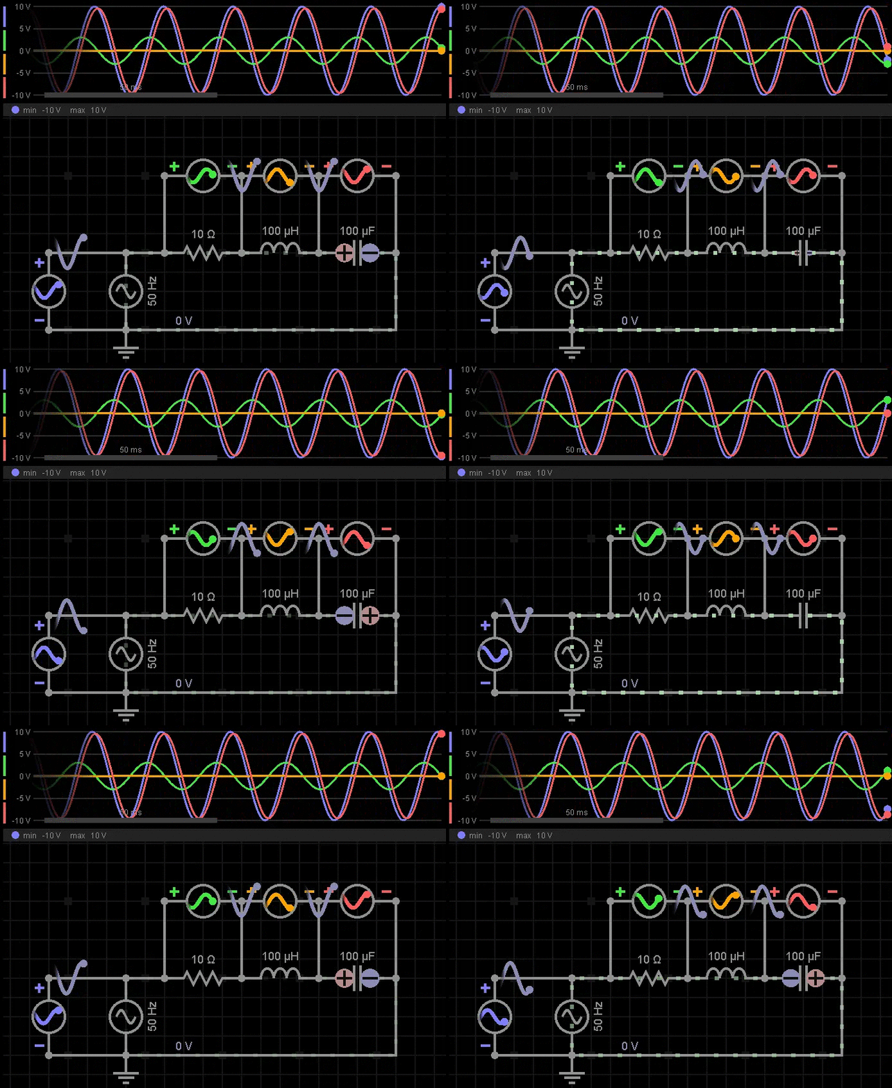
It can be seen that the peak voltage amplitudes of the three components, adding these values are greater than the peak amplitude of the power supply voltage 10V. However, in reality the voltages of the R-L-C are different in phase, at a specific point in time (t ), the sum will not be greater than the peak amplitude of the power supply voltage. 

Let’s take a look at the simulation waveform and experience the fluctuation of voltages on each component:

* Impedance Calculation Example - Circuit Simulation Waveform

What happens when the input signal is at the resonant frequency?

Through the above explanation, when calculating the circuit impedance, you will first find the difference between XL (inductive reactance) and XC (capacitive reactance) to obtain the X (reactance) of the circuit. If XL= XC, then X is 0. To achieve this goal, it is necessary to meet the formula 2π*fL = 1/(2π*fC), then get f = 1/(2π*(LC)^1/2):

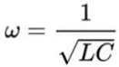
Where, ω=2πf

f=Resonance frequency, hertz

L=Inductance, Henry

C=Capacitance, Farad

ω is called the resonance frequency, which is determined by L and C in the circuit.

When the frequency of the input signal is consistent with ω, the impedance of the circuit shows pure resistance characteristics, and |Z| is minimum, and the combination of the two components L and C is equivalent to a short circuit for the input signal of this frequency.

Finally, you can calculate that the resonant frequency is about 1.592KHz, and use it as the power frequency. Please see the simulation waveform as follows:

* Resonance Frequency - Circuit Simulation Waveform

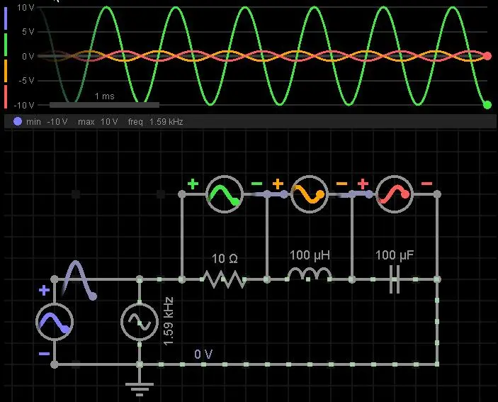
It can be seen that the voltage polarities on L and C cancel each other out, so the combination of L and C is equivalent to a short circuit. Look at the following figure, with the resonant frequency, the maximum voltage is obtained from the resistor. Of course, this is the case when RLC is connected in series. When it a parallel circuit, what happens when the resonance frequency is used as the input? You can find out below.

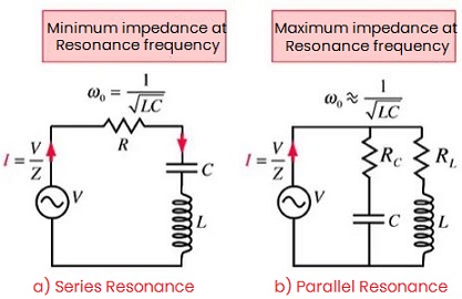
Figure 5: RLC Equivalent Circuit with Resonance Frequency (minimum and maximum impedance)

RLC Circuit Formula

1. Introduction

The RLC circuit is actually a second-order circuit. The following figure shows a series connection:

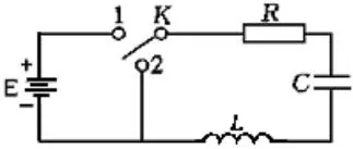
Figure 6: RLC Circuit (series)

It can be described by the following linear second-order ordinary differential equation:

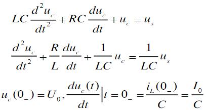
Solve the differential equation to get , and then obtain  i_C(t) based on 

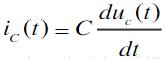
The zero input response and zero state response of the RLC series circuit are related to the coefficients of the differential equation, that is, the component parameters.

Damping coefficient description: For example, for a second-order system, the standard form of its characteristic equation is:

ζ is the damping coefficient, and ωn is the undamped oscillation frequency.

,   

The equation can be written as: 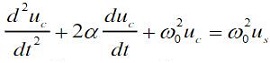, and α=ζωn

1) ζ>1, S1 and S2 are different real roots, and the response of u(t) is non-oscillatory, which is called overdamped response.

2) ζ=1, S1 and S2 are two equal negative real roots, which are called critical states.

3) ζ<1, S1 and S2 are a pair of conjugate complex roots, which is called an underdamped state.

2. Zero Input Response

In Figure 7, the initial conditions are that the capacitor voltage UC is equal to U0 and the inductor current I is equal to 0, then the switch is turned from left to right. Depending on the circuit parameters, there are four situations of zero input response:

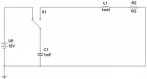
Figure 7: RLC Circuit  (Zero Input Response)

(1) When  ζ>1, the current in the circuit never changes direction during the discharge process, and the capacitor discharges non-oscillatingly all the time. The corresponding waveform is shown in Figure 8.

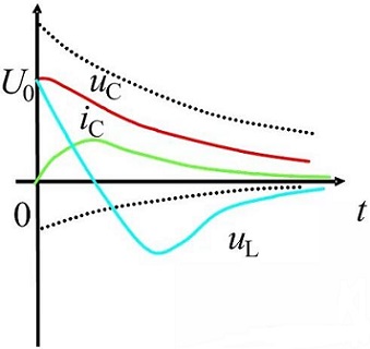
Figure 8: Overdamped Zero Input Response Waveform

(2) When  ζ=1, the capacitor discharges non-oscillatingly, and the waveform is similar to overdamping, as shown in Figure 9.

(3) When ζ<1, the capacitor voltage performs attenuated oscillation discharge near zero value, so does the current. The corresponding waveform is shown in Figure 9.

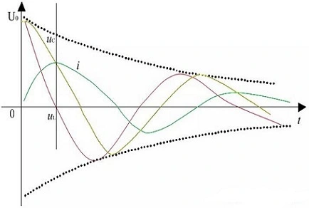
Figure 9: Zero Input Response Waveform

(4) Without damping, R=0, the capacitor voltage oscillates with constant amplitude according to the sinusoidal law. The corresponding waveform is shown in Figure 10. In reality, the damping R cannot be 0, so this phenomenon does not exist.

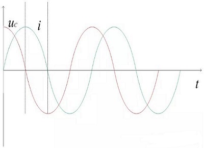
Figure 10: Undamped Zero Input Response Waveform

3. Zero State Response

The RLC circuit with zero state response is shown in Figure 11. The initial condition is that the capacitor voltage UC and the inductor current I are both equal to 0, and then the excitation is input. Like the zero-input response, there are four cases of zero-state response:

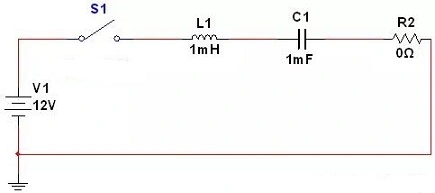
Figure 11: RLC Circuit  (Zero State Response)

(1) When  ζ>1, the current never changes direction during the charging process, and the capacitor is charged non-oscillatingly all the time. The corresponding waveform is shown in Figure 12.

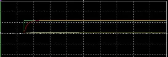
Figure 12: Overdamped Zero State Response Waveform

(2) When  ζ=1, the capacitor is charged non-oscillatingly, and the waveform is similar to over-damping as shown in Figure 12.

(3) When ζ<1, the capacitor voltage performs attenuated oscillation charging near the power supply voltage value U0, but will not exceed 2 times the power supply voltage, and the current performs attenuated oscillation near the zero value. And the corresponding waveform is shown in Figure 13.

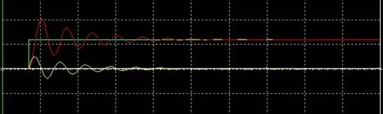
Figure 13: Underdamped Zero State Response Waveform

(4) Without damping, R=0, the capacitor voltage oscillates with constant amplitude around the power supply voltage value U0 according to the sinusoidal law between 0 and 2 times the power supply voltage, and the current oscillates with constant amplitude around the zero value. The angular frequency is, and the corresponding waveform is shown in Figure. In reality, the damping cannot be 0, and this phenomenon does not exist.

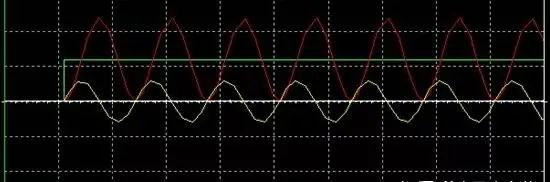
Figure 14: Underdamped Zero State Response Waveform

RLC Oscillation Explained

In the circuit, the capacitor voltage is continuous and cannot change suddenly. The capacitance formula I=Cdu/dt can be converted to du=Idt/C.

According to the derivative knowledge, the derivative of a continuous function at the extreme point is equal to 0, so when the capacitor voltage value is maximum, that is, the voltage derivative du=0, Idt/C=0, the capacitor current I=0 can be obtained. Similarly, the inductor current is continuous and cannot mutate, and the inductor formula is U=Ldi/dt. When the inductor current is maximum, the inductor voltage UL is 0.

* Zero Input Response

In Figure 15, the initial condition is that the capacitor voltage is U0 and the inductor current is 0. Since the resistance R=0, according to Kirchhoff's voltage law, the inductor voltage UL is equal to the capacitor voltage UC. At time 0, because the capacitor voltage is U0, the charges on both sides of the plates are unbalanced, and the polarity is positive up and negative down, so the capacitor begins to discharge, and the current in the circuit begins to increase, and the flow direction is clockwise. Until t1, the capacitor is completely discharged and the voltage UC is 0, so the inductor voltage UL is 0.

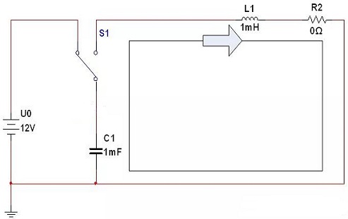
Figure 15: Current Direction (Zero Input Response)

According to the above inductance characteristics, the circuit current I is maximum at this time, and the charges on both sides of the capacitor are in a balanced state. Although the capacitor is in a charge balance state at time t1, the inductor current cannot mutate and cannot change from the maximum value to 0 instantly, but decrease slowly. This causes the charge balance state of the capacitor to be broken, the capacitor is recharged, and the polarity is different at t0, that is, it is negative up and positive down, until I=0 at t2. According to the above capacitor characteristics, the capacitor voltage reaches the maximum value at this moment, but the charges on both sides are in an unbalanced state again; then begins to discharge, and the current direction is opposite to that in the 0~t1 period, which is counterclockwise. In addition, the phase difference between the capacitor voltage and current in the entire process is exactly 90°.

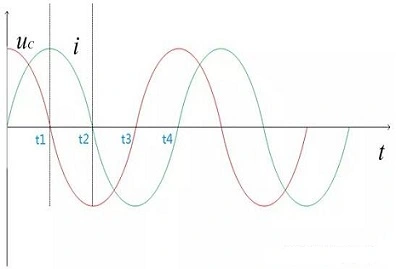
Figure 16: Undamped Zero Input Response Waveform Analysis

When the damping resistance R≠0 in the circuit, the waveform is as shown in Figure. Since the R has a voltage drop UR, the inductor voltage UL is not equal to the capacitor voltage UC, but meets the following relationship: UC=UL+UR. At time 0, the capacitor discharges, the capacitor voltage UC drops, the current I increases, and the resistor voltage UR increases. At t1, UC and UR are equal, that is, UC=UR=IR, the inductor voltage UL is equal to 0, and I reaches the maximum value, I=UC/R, which is smaller than the maximum current value in the undamped state.

The capacitor has not yet completely discharged at t1, so it continues to discharge until the end at t2. The inductor current reaches its maximum value at t1 and then begins to decrease, but the current direction remains unchanged. Until t2, the capacitor voltage is completely discharged, the inductor current begins to charge the capacitor, and the capacitor polarity changes to negative up and positive down, by t3, I=0, the capacitor voltage UC reaches the maximum value. It can be seen from the analysis that due to the existence of the resistor R, the inductor current has reached the maximum value before the capacitor is fully discharged. The larger the resistor R, the smaller the maximum current value I=Uc/R, and the shorter the time when the current reaches the maximum value. When , the current and capacitor voltage both reached 0 at the same time and stopped oscillating, forming a non-oscillatory discharge.

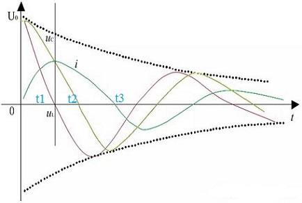
Figure 17: Underdamped Zero Input Response Waveform Analysis

* Zero State Response

The initial conditions of the capacitor voltage UC and the inductor current I are both 0, and the excitation voltage is U0. At t0, the capacitor begins to charge, and the capacitance UC and I begin to increase. Until t1, the capacitor voltage UC rises to U0, at this time, the inductor voltage UL=0 and I reaches the maximum value. After t1, I begins to decrease, but the direction remains unchanged, and the capacitor continues to charge until t2, the current drops to 0 and the capacitor voltage UC reaches the maximum value 2U0. After t2, the capacitor begins to discharge, the current direction changes to the opposite direction. Until t3, the capacitor voltage UC drops to U0, UL=0, and the inductor current reaches the maximum reverse value.

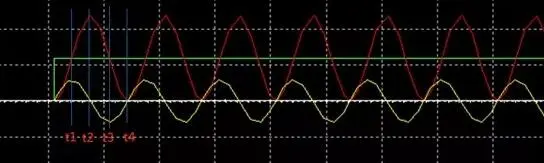
Figure 18: Undamped Zero State Response Waveform (t1-t4)

When the damping resistor R≠0 in the circuit, due to the voltage drop in the resistor, U0=UR+UC+UL, the waveform is shown in Figure. At t0, the capacitor begins to charge, and UC and I begin to increase. Until t1, U0=UR+UC, UL=0, and the current reaches the maximum value,  I=(U0-UC)/R, which is less than the maximum current in the undamped state, and the inductor current begins to decrease after t2. When UC, until t2, the inductor current drops to 0, and the capacitor voltage reaches the maximum value, which is smaller than the value in undamped state. After t2, the capacitor begins to discharge, and the current direction becomes opposite. Until t3, U0=UC+UR, the current reaches the maximum value in the opposite direction, at this time UC>U0, the capacitor voltage has not yet dropped to U0. During t3~ t4, the current gradually decreases from the reverse maximum value to 0. At t4, the current is 0 and the capacitor voltage reaches the minimum value. At this time, UL=Ldi/dt>0, UR=0, U0=UL+UC, U0>UC. Because the inductor current cannot suddenly change and start charging the capacitor, and some energy is consumed by the resistor, the peak current value becomes smaller and smaller.

From the analysis, it can be seen that the larger the resistor R, the larger the damping value, and the damping has the effect of returning the circuit to a stable state from oscillation, the smaller the current maximum value I=(U0-UC)/R, the earlier the moment when the current reaches the maximum value, the capacitor voltage can reach the maximum value is also smaller. At that time, the maximum value reached by the capacitor voltage when the current is 0 is close to equal to U0. Since there is no voltage difference between the capacitor voltage and the excitation source U0, it cannot be charged or discharged again, eventually forming a non-oscillating charge.

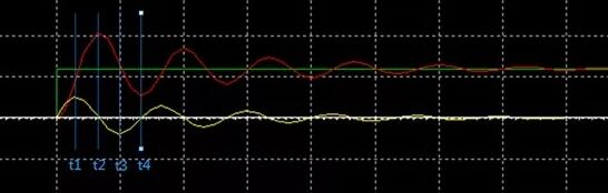
Figure 19: Underdamped Zero State Response Waveform (t1-t4)

In short, the RLC circuit to oscillate is that the capacitor or inductor is in an unstable state, that is, the capacitor can charge or discharge, and the current flowing through the inductor is not 0, and  the final stable state must be that the capacitor does not have the ability to charge or discharge conditions.